Finite Element Analysis Operations
Mesh Generation
To generate a shell model without adhesives in ANSYS simply type:
>> includeAdhesive=0; >> meshData=blade.generateShellModel(‘ansys’,includeAdhesive)
The function returns a struct that contains the following feilds: nodes, elements, outerShellElSets, and shearWebElSets. This struct later needs to be input into mainAnsysAnalysis.
Coordinate Systems
Loading for the FEA model will typically be derived from FAST or OpenFAST cross-sectional stress resultant forces and moments at various spanwise positions. These forces and moments are in coordinate systems that are aligned with the local principal axes (structural) of the cross-section in the deformed configuration. Thus, those coordinate systems change with respect to span. Fig. 2 contrasts the FAST results coordinate basis vectors, \(v_{i}^{(j)}\ (j = 1,2,3,\ldots,k)\), with those of the NuMAD loads system, \(w_{i}\), and the ANSYS coordinate system, \(x_{i}\), which are invariant. \(v_{i}^{(j)}\) is the also known as the blade coordinate system in FAST/OpenFAST. Here and through the rest of this document, index notation is used with Latin indices assuming 1, 2, and 3 and Greek indices assuming 1, and 2 (except where explicitly indicated). Repeated indices are summed over their range (except where explicitly indicated).
Note
The \(x_{i}\) coordinate system is like the \(w_{i}\) system but the first axis, \(w_{1}\) points toward the leading edge instead of the flap direction.
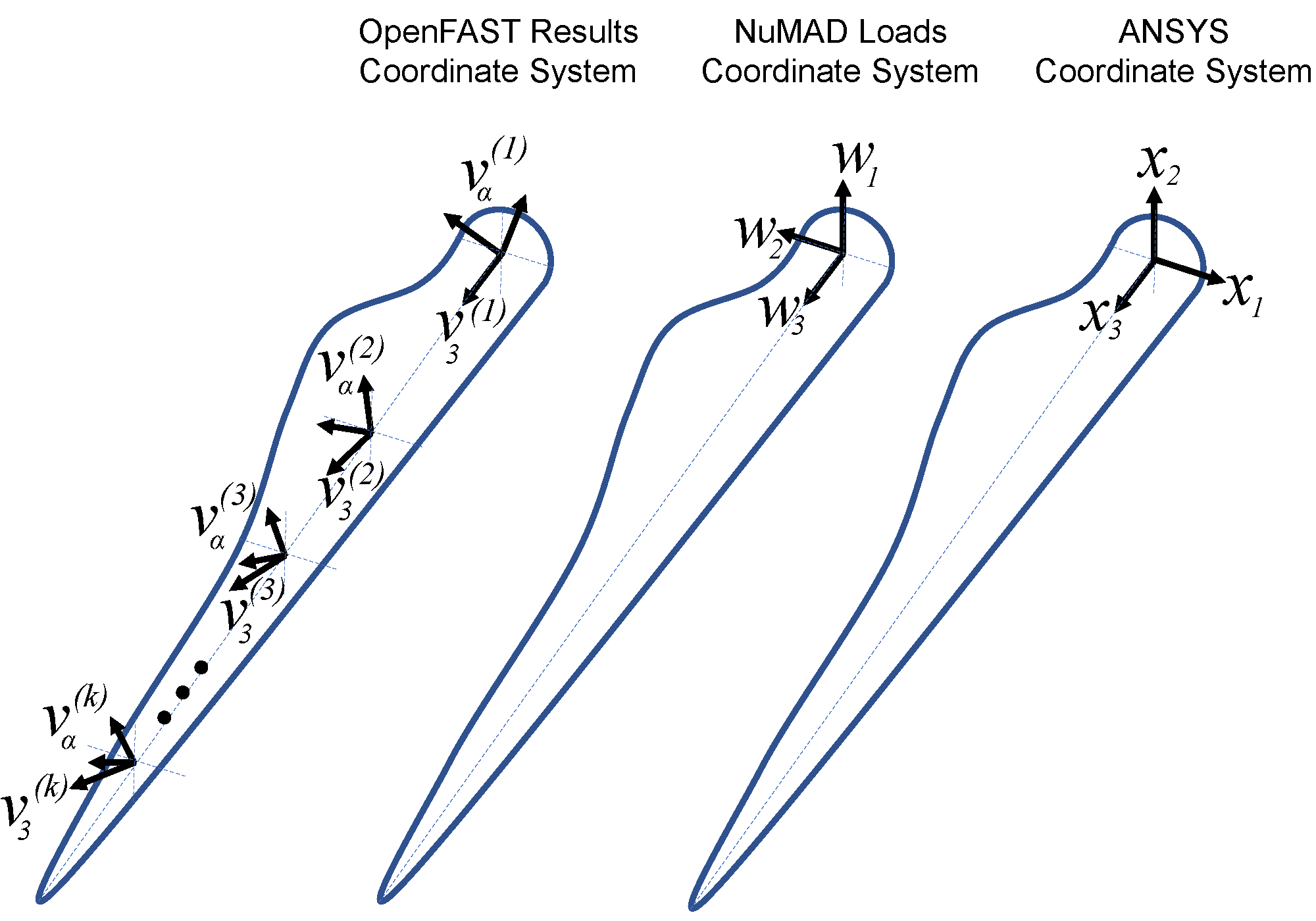
Fig. 2 Comparison of the FAST results coordinate system with that of the NuMAD and ANSYS coordinate systems.
A small angle is assumed to exist between \(v_{3}^{(j)}\ (j = 1,2,3,\ldots,k)\) and \(w_{3}\) and is unaccounted for in NuMAD. Thus, it is assumed that \(v_{3}^{(j)} = w_{3} = x_{3}\). Thus the \(v_{i}^{(j)}\) and the \(w_{i}\) are related by
where \(C_{iq}\) are the direction cosines which can be stored in a matrix as shown below
where \(\mu\) is the so-called structural twist and is illustrated in Fig. 3.
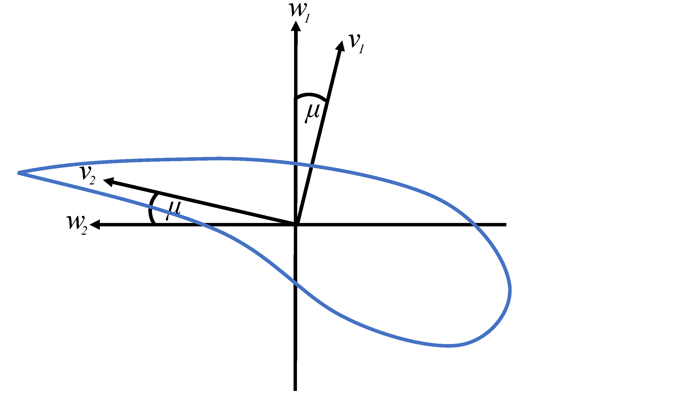
Fig. 3 Time history moment data from the \(v_{\alpha}\) coordinate system to the \(w_{\alpha}\) intermediate coordinate system.
These angles are obtained by PreComp. This coordinate transformation is
implementation in loadFASTOutDataGageRot.
Before transforming the loads data to the \(x_{i}\) system, various data processing operations occur in intermediate coordinate systems as described in the next section.
Analysis Directions
Increasing the fidelity from a beam model in FAST/OpenFAST to a shell model also increases the computational cost. Thus, it would be cumbersome to conduct a time history structural analyses with a shell model for each DLC; it would be impracticable on each iteration of an optimization loop. Therefore, it is necessary to construct a reduced set of load cases that is representative of the most critical loads in the time history analysis.
Two load cases were deemed necessary to properly analyze the most critical loads; those needed to evaluate the maximum tip deflection and those needed for evaluating blade failure. Here, blade failure consists of ultimate failure, buckling, and fatigue failures. Both cases utilize the FAST/OpenFAST resultant axial forces \(F_{3}^{w}\), both bending moment components \(M_{\alpha}^{w}\), and the twisting moment, \(M_{3}^{w}\). The superscript indicates the reference frame. These will be referred to collectively with \(P_{i}\ (i = 1,2,\ldots,4)\), a generalized load vector, where \(P_{i} = \begin{bmatrix} F_{3}^{w} & M_{1}^{w} & M_{2}^{w} & M_{3}^{w} \\ \end{bmatrix}^{T}\).
Note
Note that \(P_{i}\) varies with span-wise location and that resultant shear forces were assumed to be negligible for establishing load equivalency for both load cases.
For the tip deflection case, the time at which the maximum tip deflection from the beam model, \(t^{*}\ \), was determined. Then the \(P_{i}\), at a given cross section was defined by
The components were then transformed to the \(x_{i}\) system.
Since IEC allows for lower factors of safety if numerous analysis
directions are considered, \(n_{\theta}\) analysis directions can be
considered by setting momentMaxRotation to \({n}_{\theta}\)
in the IECInput.inp file.
Thus the loads used to evaluate blade failure are obtained by letting \(\theta\), as defined in Fig. 4, vary from 0 to 360 deg. in increments of \(n_{\theta}/360\); yielding \(n_{\theta}\) FE load cases. The results for the load directions 0\(\leq \theta\)<180 deg. were obtained by
\(P_{i} = \begin{bmatrix} \text{max}(F_{3}^{w}(t)) \\ \text{max}(M_{1}^{y}(t))\cos(\theta) \\ \text{max}(M_{1}^{y}(t))\sin(\theta) \\ \text{max}(M_{3}^{w}(t)) \\ \end{bmatrix}\) 0\(\leq \theta\)<180
where
Load directions from 180\(\leq \theta\)<360 deg. are, however, obtained by
\(P_{i} = \begin{bmatrix} \text{max}(F_{3}^{w}(t)) \\ \text{min}(M_{1}^{y}(t))\cos(\theta) \\ \text{min}(M_{1}^{y}(t))\sin(\theta) \\ \text{max}(M_{3}^{w}(t)) \\ \end{bmatrix}\) 0\(\leq \theta\)<180
Note
In the above equation, the minimum of \(M_{1}^{y}\) is found
instead of the maximum but \(\theta\) still ranges from 0 to 180 deg.
Unlike the resultants used for the deflection analysis which all occurred
at a specific time in the OpenFAST simulations, each of the axial force,
torsion, and bending moment resultants along the span could possibly come
from different times. Thus, it is an artificial distribution suitable for
design use. Also unlike the deflection case, the two bending-moment
components (i.e. flap-wise and edge-wise bending) at a span location
were projected onto 12 directions as defined by \(y_{1}\) in
Fig. 4. All of the \(P_{i}\ \)then transformed
to the \(x_{i}\) system in beamForceToAnsysShell.
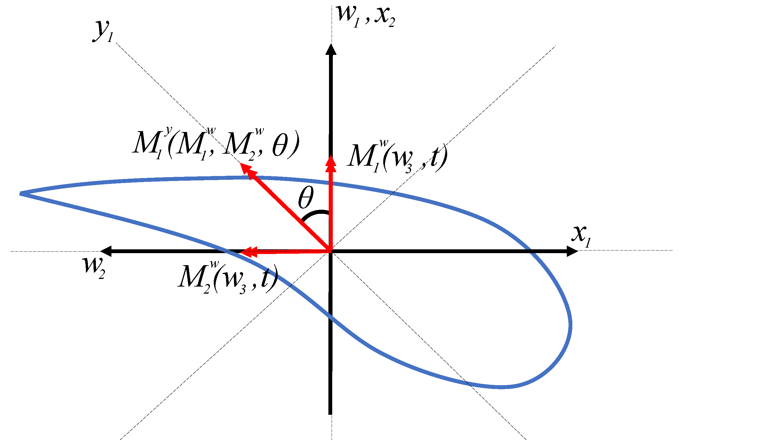
Fig. 4 The definition of the \(y_1\) axis and the angle \(\mathbf{\theta}\).
Loads Application
Blade loads can either come from the cross-sectional stress resultant
time-histories from FAST or user defined. Two load types are supported
for loads coming from a FAST; loads at a particular time and extremum
loads used to evaluate the limit states of the blade. Both account for
all three cross-sectional resultant moments along the span as well as
the resultant axial forces. However, the resultant transverse shear
forces acting on the blade in the FAST model are not transferred the
ANSYS model. Moreover, both create the loadsTable variable needed by
mainAnsysAnalysis, the main FEA script described is subsequent
section. getForceDistributionAtTime.m handles can be called for the
loads at a given time while FastLoads4ansys.m} builds the loadsTable for
each analysis direction. The loadsTable variable
is\(\ 1 \times n\) MATLAB cell array where \(n\) is
the number of analysis directions.
Note
getForceDistributionAtTime.m will give a \(1 \times 1\) cell array since the loading is the actual loading at a particular time.).
A user may apply loads other than the loads at particular time or the extremum loads with a user
defined loadsTable. This can be done by creating the structure of the
loadsTable variable manually.
Example use for FastLoads4ansys.m is as follows:
%Get extremum loads
fast_gage=get_fast_gage(params.momentMaxRotation);
output=layupDesign_FASTanalysis(blade,'1.3',0,0);

% Loads to be applied to blade
halfdz=2.5; %for best results halfdz should be a multiple of L and should be <= L/2

bladeLength = blade.ispan(end);
r=2.5:5:bladeLength; %Location where output forces and moments will be calculated

loadsTable = FastLoads4ansys(output,fast_gage,r);
For bending moments on a blade, getForceDistributionAtTime.m and
getForceDistributionAtTime.m convert the moment distributions to
transverse force distributions. Fig. 5 shows the known spanwise
bending moments, \(M_{i}\) acting at a distance \(z_{i}\) from
the blade root and the forces to be solved, \(F_{i}\) acting at
\({\overline{z}}_{i}\), where
\({\overline{z}}_{i} = 1/2(z_{i} + z_{i + 1})\).
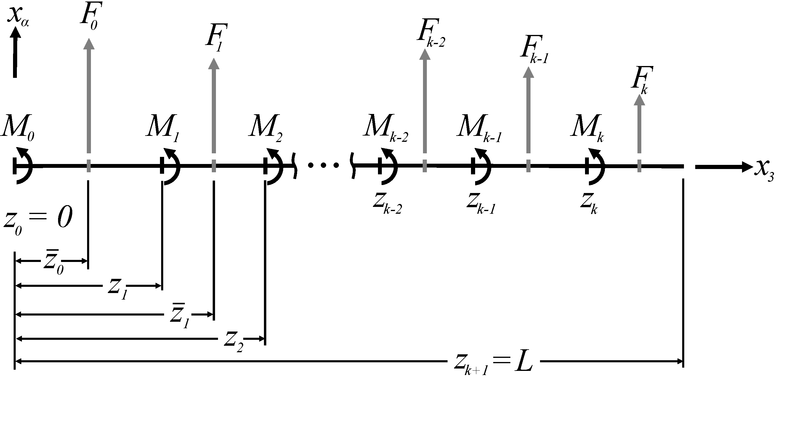
Fig. 5 Freebody diagram used to determine transverse loads from a given distribution of moments along the blade span.
From static equilibrium, the forces to be applied are found by solving the following linear system of equations for \(F_{i}\ (i = 1,2,3,\ldots,k)\)
where \(k\) is the number of cross-sections with resultant moment data.
The load distributions are then transferred to nodal loads by
beamForceToAnsysShell.m. beamForceToAnsysShell.m generates a text file (usually called forces.src)
containing the APDL commands to apply nodal forces for every node on the
wetted area of the blade. Details of the approach are found in Ref. [1]
but with modifications to add axial loads.
Note
The script assumes that the input forces are in the FAST coordinate system, \(w_{i}\), so a conversion is performed in the script to the ANSYS coordinate system, \(x_{i}\).
A vector, \(G_{i}\), such as a force or a moment, in the \(w_{i}\) coordinate system is transformed to the \(x_{i}\) with
where \(C_{ij}\) is defined in Eq. (4) but with setting
\(\mu = - 90\ \)deg. Example usage for the first loadsTable load
case is as follows
output=layupDesign_FASTanalysis(blade,DLCoptions,runFASTAnal,useParallel)
loadsTable =FastLoads4ansys(output,fast_gage,r)
beamForceToAnsysShell(maptype,nlistfile, loadsTable{1},outfile)
where maptype is either 'map2D_fxM0' or 'map3D_fxM0'. Note that these
steps are not usually required with using mainAnsysAnalysis, the
main analysis script. These instructions are for building the loadsTable variable
and applying nodal forces to an FE model in a stand-alone manner.
Analysis Script
mainAnsysAnalysis.m is the main analysis script. A user may call
on it to
obtain load factors from global instabilities due to linear or nonlinear buckling
obtain load factors from local instabilities due to face-sheet wrinkling
find the maximum value of a failure index
stress data required for fatigue analyses
cross sectional force and moment results vs spanwise position
average cross-sectional rotations and displacements along the span
strain along the spar caps vs. spanwise position
blade mass
The required inputs are a blade object, the loadsTable, and the config
variable. The script knows which analysis types it should run based on
config. See Table 3 for the structure and usage of the config
variable. The IECDef class defintion is only needed when the fatigue flage is activated.
Field Name |
Example Value |
Activation Logic |
|---|---|---|
|
|
If Field Name exists and is not empty. |
|
|
If Field Name exists and is not empty. |
|
1 |
If Field Name exists and is not empty. Defaults to 1. |
|
3 |
If Field Name exists and is greater than 0. |
|
0 |
If Field Name exists and is not empty. |
|
|
If Field Name exists and is not empty. |
|
|
If Field Name exists and is not empty. |
|
|
If Field Name exists and is not empty. |
|
1 |
If Field Name exists and is not equal to 0. |
|
1 |
If Field Name exists and is not equal to 0. |
|
|
If Field Name exists and is not empty. |
|
1 |
If Field Name exists and is not empty and is not equal to 0. |
meshFile is the name of the ANSYS model database to begin the analysis
from. It defaults to 'master'. analysisFileName is the name of the new
ANSYS model database which will store the analysis results. It defaults
to 'FEmodel'. np is the number of processors (CPUs) ANSYS should use for
each solve. It defaults to 1.
The output and it is a variable length struct. Depending on which analysis flags are active, results can be accessed with
>> result=layupDesign_ANSYSmesh(blade)
>> result.globalBuckling
>> result.localBuckling
>> result.deflection
>> result.failure
>> result.fatigue
>> result.resultantVSspan
>> result.mass
Linear-Static Analysis
A linear-static analysis is defined and solved by default. Since linear-buckling is a notable advantage of using a shell model for the blade, prestress is activated in this load step in preparation for a linear buckling analysis. The effects of inertia are counterbalanced with inertia relief.
Depending on the config flags, a number analysis outputs can be
examined.
Deflection
Setting config.deflection = 1 will cause result.deflection to
hold the average deflection of each cross-section at every blade.ispan
location. For example, access results from the second loadsTable case as
result.deflection{2}
The result is a matrix that has as many rows are blade.ispan and 6
columns. The first three columns are average cross-sectional
displacements in the \(x_{i}\) system. Columns 1, 2, and, 3,
correspond to \({\overline{u}}_{1}\), \({\overline{u}}_{2}\),
and \({\overline{u}}_{3}\) respectively. Columns 4, 5, and 6
correspond to \({\overline{\theta}}_{1}\),
\({\overline{\theta}}_{2}\), and \({\overline{\theta}}_{3}\),
respectively.
Failure
If material failure is being considered in an analysis, set
config.failure equal to any one of the entries in Table 4. An
empty string will skip any material failure analyses.
Failure Criterion Type |
|
|---|---|
Maximum Strain |
|
Maximum Stress |
|
Puck Failure |
|
LaRC03 |
|
LaRC04 |
|
Tsai-Wu |
|
Depending on the criterion used, it is necessary for the materialDef to
have the appropriate material properties defined in blade.materials.
Since each element section is a layered composite, by default,
result.failure will hold the maximum failure index of all elements and
every layer.
Global Buckling
A nonzero number for config.analysisFlags.globalBuckling will call
ANSYS to run a buckling analysis. The buckling analysis can either be
linear or nonlinear. The nonlinear case will be activated by creating
config.analysisFlags.imperfection and setting it to a nonempty
number array. ANSYS will then be directed to perform an eigenvalue
buckling analysis. The load which results in nonconvergence will be
reported as the nonlinear buckling load factor.
For the nonlinear case, it is necessary to introduce a synthetic imperfection for the analysis to provide reasonable results. The imperfection introduced is of the geometric kind and corresponds to the buckled mode shapes obtained in the eigenvalue buckling analysis. Therefore, an eigenvalue buckling analysis precedes the nonlinear static analyses. Currently, for nonlinear buckling, it is assumed here that buckling will be in the aeroshell (not the web). Thus, each mode shape is scaled such that the maximum displacement in the \(x_{2}\) direction (flapwise) is equal to config.analysisFlags.imperfection in value. Robustness could be increased if the script can select whether to find the maximum displacement in the \(x_{2}\) (buckling in aeroshell) or \(x_{1}\) direction (buckling in the webs).
Finally, it is supposed that the mode shape corresponding to the lowest load factor from the eigenvalue analysis will not always cause the lowest load factor from the nonlinear case. Thus, a nonlinear static analysis for each requested mode is performed and the minimum load factor is reported.
Local Buckling
Sandwich panels typically consist of a relatively soft core layer sandwiched between two faces sheets. For the parts of blade that are described as sandwhich panels, local instabilities can be checked in NuMAD with a strip theory model from Ref. [2]. In particular, this check examines if the outermost facesheet wrinkles under compression.
To activate this check, set config.analysisFlags.localBuckling
equal to the name of the core material in your BladeDef as a string
(e.g. config.analysisFlags.localBuckling = 'Balsa'). Otherwise an
empty string will skip the analysis. Currently, all ply angles are
limited to zero (i.e. no off-axis layups).
Fatigue
If config.fatigue is a nonempty string, then ANSYS will be
directed to write model data and field output to text files for fatigue
post-processing in MATLAB. Namely, Elements.txt, Materials.txt,
Strengths.txt, Sections.txt, and plate strain measures. The results from running
the fatigue post-processor will be a \(1 \times n_{\theta}/2\) cell
array, where \(n_{\theta}\) is the number of cells in the loadsTable
variable (where each cell holds the loads for a single analysis
direction). This is because stress results from two orthogonal loading
directions are utilized for a single evaluation of fatigue damage (e.g.
one fatigue evaluation is the combined effect of flap loads and edge
loads). Furthermore, it assumes that the loadsTable is arranged in
ascending order for the loads direction angle. This is already accounted
for if loadsTable was constructed from FastLoads4ansys.m.
Make sure to set fatigueCriterion to Shifted Goodman
in the IECInput.inp file.
Fatigue damage is computed at the root and at the locations of the FAST gages. In this document, these will be referred to as the spanwise fatigue locations. Fatigue results are restricted to the spanwise fatigue locations because the fatigue analysis relies on Markov matrices and these matrices need cycle counts from time-history data. The time histories that are available from FAST are at the root and the FAST gages.
The end-user has the ability to either obtain a single fatigue damage
fraction at each spanwise fatigue location or several fatigue damage
fractions each corresponding to a region in Fig. 1. The former is
accomplished by setting config.analysisFlags.fatigue = ["ALL"].
The latter is accomplished by setting config.analysisFlags.fatigue
to a MATLAB string array where any and all Region Names in Table 5 are allowed.
Region Name |
Region Description |
|---|---|
|
High pressure trailing edge flatback |
|
High pressure trailing edge reinforcement |
|
High pressure trailing edge panel |
|
High pressure spar cap |
|
High pressure leading edge panel |
|
High pressure leading edge |
|
Low pressure leading edge |
|
Low pressure leading edge panel |
|
Low pressure spar cap |
|
Low pressure trailing edge panel |
|
Low pressure trailing edge reinforcement |
|
Low pressure trailing edge flatback |
|
All webs |
For example, suppose that the fatigue damage was only desired at the spar caps and the reinforcement locations one would set
>> config.analysisFlags.fatigue = ["HP_TE_FLAT","HP_TE_REINF","HP_SPAR","HP_LE","LP_LE","LP_SPAR","LP_TE_REINF","LP_TE_FLAT"]
If "ALL" is included along with other regions, the other regions are
ignored and the analysis carries forth as it would for "ALL".
The result will be a \(1 \times n_{\theta}/2\) cell array. Each cell
will hold a struct with the following field names: fatigueDamage,
criticalElement, criticalLayerNo, and criticalMatNo. Each of these field
names allow access to a \(n_{\text{region}} \times 10\) matrix where
\(n_{\text{region}}\) is the length of
config.analysisFlags.fatigue. The results are organized such that
the \(i_{\text{th}}\) row number corresponds to fatigue damage
results of the \(i_{\text{th}}\) Region Name from
config.analysisFlags.fatigue. The columns correspond to the
fatigue damage spanwise locations where column 1 is the results at the
root. Subsequent columns correspond to successively farther gage
locations.
The results from the first fatigue evaluation can visualized as shown in Fig. 6.
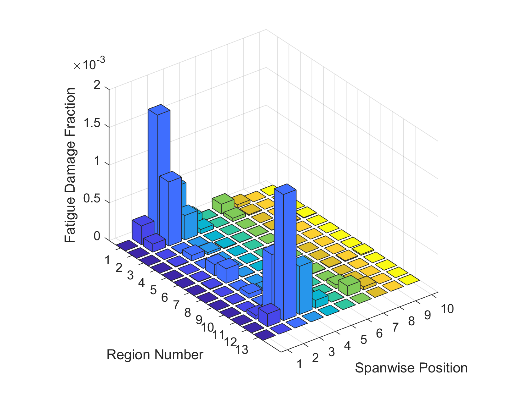
Fig. 6 Fatigue damage fraction visualization.
Local Fields
If config.analysisFlags.localFeilds is activated, then the plate
strains and curvatures for every element will be written to
plateStrains-all-1.txt.
After mainAnsysAnalysis completes execution, access the local fields with
myresult=extractFieldsThruThickness('plateStrains-all-1.txt',meshData,blade.materials,blade.stacks,blade.swstacks,elNo,coordSys)
elNo is an scalar or array of element numbers for
which to extract the local fields. Set coordSys='local' to obtain
results in the local layer coordinate system or set coordSys='global' to
obtain results in the element coordinate system.
For example if one sets elNo=[1950,2558] then, myresult is a struct with
two fields:
>> myresult
         element1950: [1x1 struct]
         element2558: [1x1 struct]
Looking at the first struct shows:
>> myresult.element1950
     x3: [8x1 double]
     eps11: [8x1 double]
     eps22: [8x1 double]
     eps33: [8x1 double]
     eps23: [8x1 double]
     eps13: [8x1 double]
     eps12: [8x1 double]
     sig11: [8x1 double]
     sig22: [8x1 double]
     sig12: [8x1 double]
     matNumber: [8x1 double]
where x3 is the thickness coordinate, eps are the strains and sig are the
stresses.
Note
Note the x3 value that is zero corresponds to the reference surface in the shell model.
In this example the shell offset in ANSYS was set to BOT so the zero appears the end:
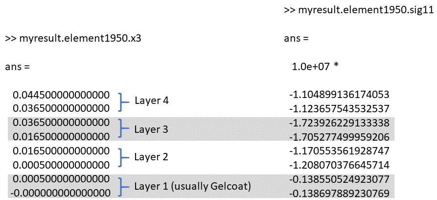
Fig. 7 Explanation of how data for local fields is ordered.
A plotting utility has been made to visualize the local fields. This can be achieved for example:
scaleFactor=1e6; %Used to plot stress in MPa and strain in microstrain
close all;
figureNumbers=[4,5];
myYlabel='$y_3$ [mm]';
plotLocalFields(figureNumbers,myYlabel,myresult.element1950,scaleFactor,'k')
plotLocalFields(figureNumbers,myYlabel,myresult.element2558,scaleFactor,'r')
legend('LE Reinf. Element','Spar Cap element')
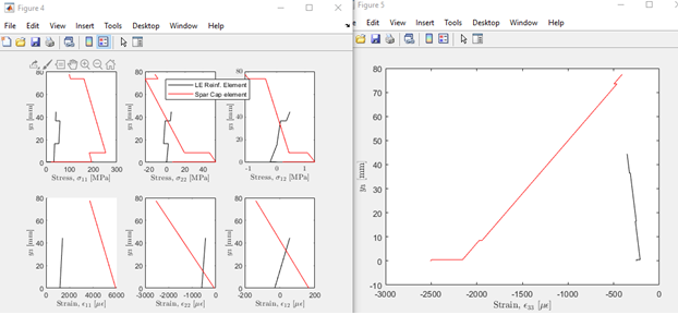
Fig. 8 Local fields example plots.
Resultant Forces and Moments
The resultant forces and moments due to stresses on cross-sections along
the span can be obtained by activating
config.analysisFlags.resultantVSspan. result. resultantVSspan{i}
will yield a \(n \times 7\) matrix, where \(n\) is approximately
equal to the blade length divided by blade.mesh. The first column is the
distance along \(x_{3}\) that locates the cross-section. The next
three columns correspond to resultant forces in the \(x_{1}\),
\(x_{2}\), and \(x_{3}\) directions (in that order). The next
three columns correspond to resultant moments about in the
\(x_{1}\), \(x_{2}\), and \(x_{3}\) directions (in that
order). For example, access results such as
>> result.resultantVSspan{i}
where i is the ith load case in loadsTable.